Louis La Minh Hoang

In this physics lesson, I studied lenses at a deeper level, with a strong focus on formulas and problem-solving, especially situations where either the object or the lens itself is moving. Instead of just drawing ray diagrams, we analyzed how image position, size, and nature change dynamically.

We began by revising the key lens equations, particularly the lens formula and magnification relationships. These formulas became the main tools for predicting how an image behaves when the object distance changes. Rather than treating the formulas as isolated rules, we used them to understand trends — for example, how moving an object closer to a convex lens affects image distance and magnification, and why certain positions lead to virtual or real images.

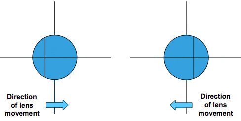
The more challenging problems involved lenses in motion. In these questions, the object or lens was gradually moved, and we had to determine how fast the image moved in response or whether the image shifted in the same or opposite direction. Solving these required careful differentiation of the lens formula and a clear understanding of sign conventions, making the problems more mathematical and less visual.

We also studied cases where the image transitions between different states, such as from real to virtual, or from inverted to upright. Identifying these critical positions required both algebraic precision and physical intuition. Some problems combined multiple ideas, such as changing magnification while keeping certain quantities fixed, which forced us to think about constraints rather than just raw calculation.

By the end of the lesson, lenses felt far more dynamic than static. The formulas were no longer just tools for finding numbers; they became a way to describe continuous change. This lesson showed how powerful mathematical analysis can be in optics, especially when understanding how small movements lead to significant changes in the final image.